About this website
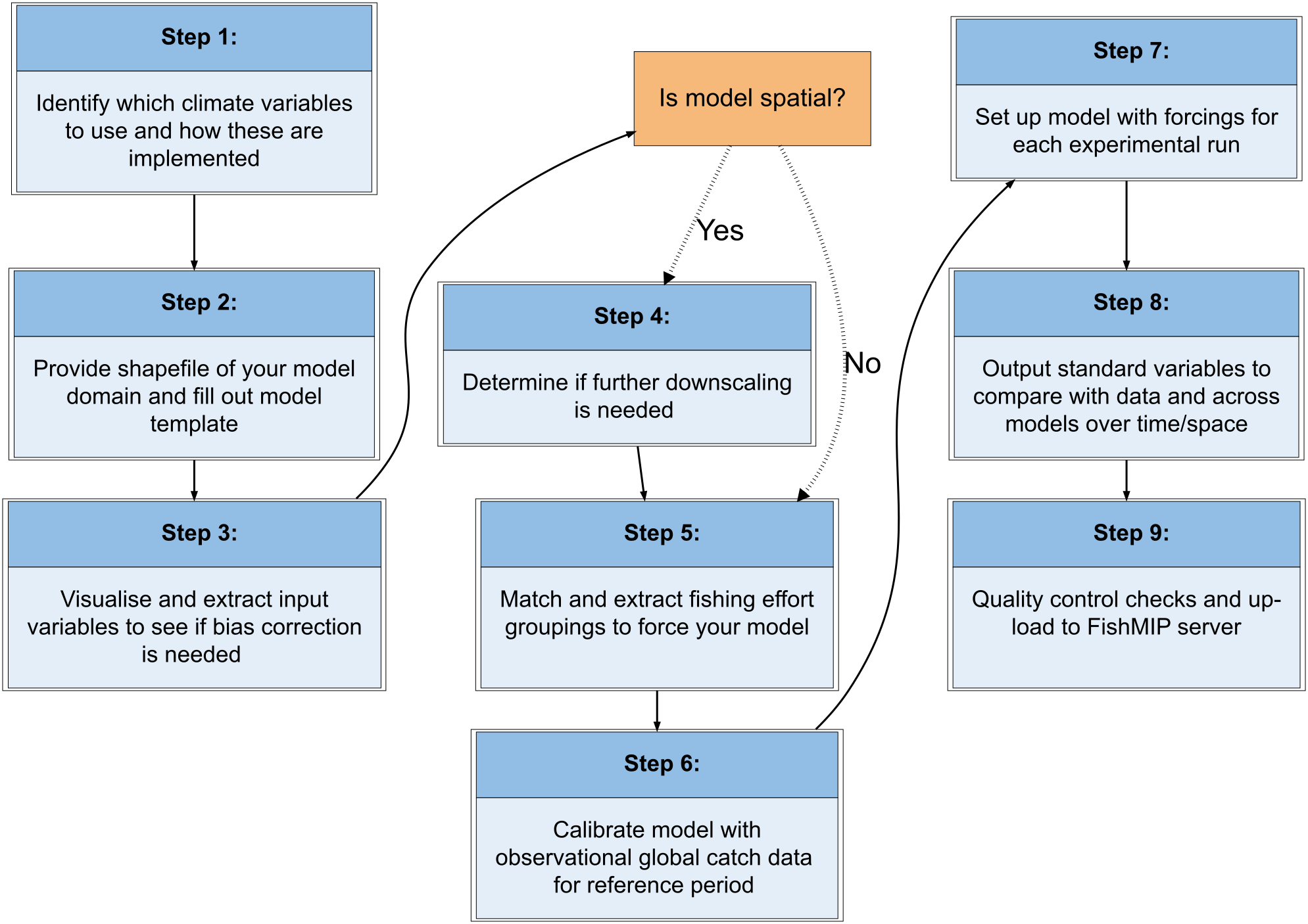
This tool allows regional modellers to visualise
environmental data from GFDL-MOM6-COBALT2 and from
observations to determine if bias correction (Step 3 below)
needs to be applied to the data prior to its use as forcings of
a regional marine ecosystem model.
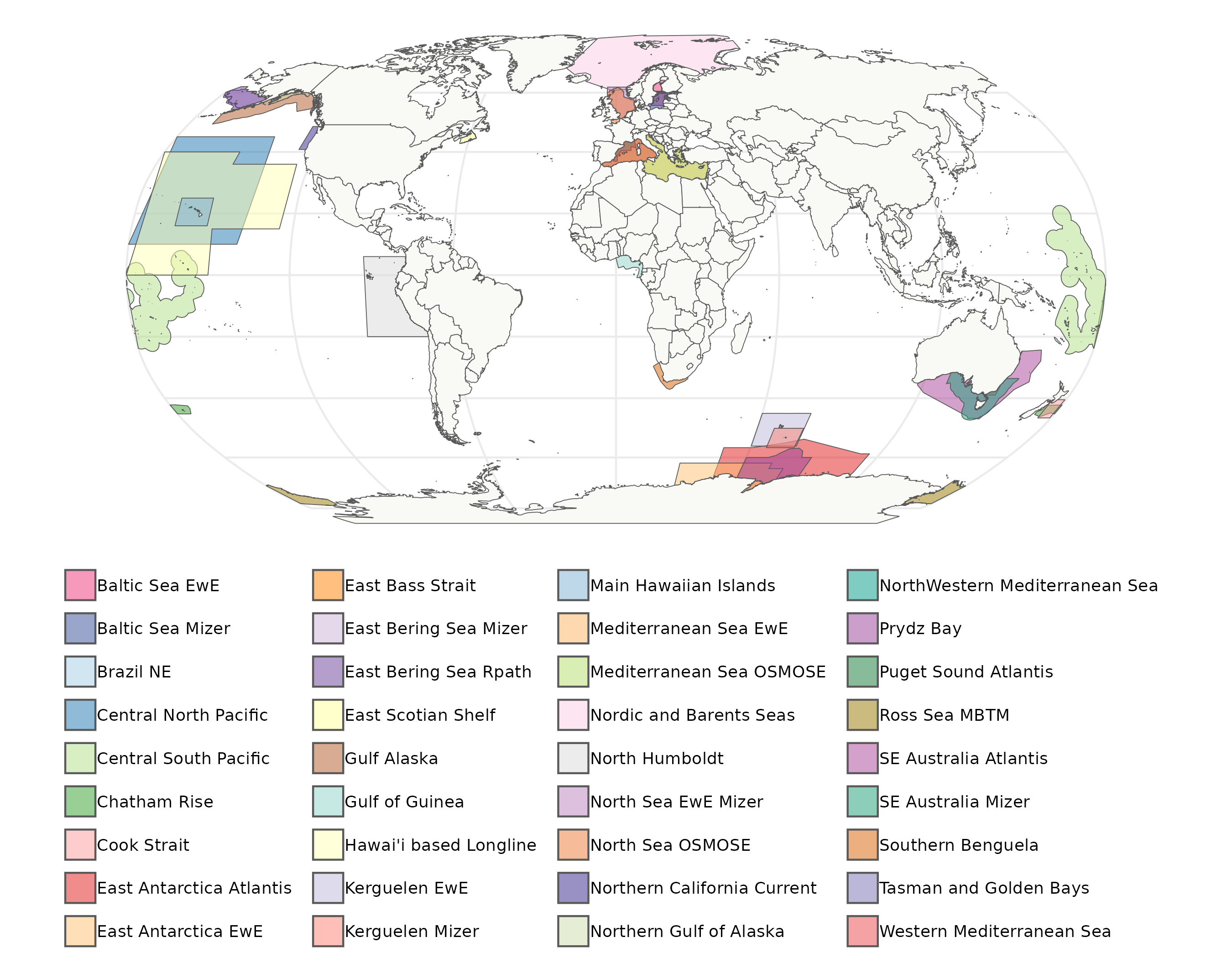
Who is FishMIP?
The Fisheries and Marine Ecosystem Model Intercomparison
Project (FishMIP) is an network of more than 100 marine ecosystem
modellers and researchers from around the world. Our goal is to
bring together our collective understanding to help better
project the long-term impacts of climate change on fisheries and
marine ecosystems, and to use our findings to help inform policy.
You can find more information about FishMIP on our
website.
How should I use this tool?
This site has three main tabs:
1.
GFDL model outputs:
Here you can
download the GFDL-MOM6-COBALT2 ocean outputs as originally
available in the
ISIMIP data repository.
Data available for download in this tab has not been
processed in any way, we have simply extracted all available
data within the boundaries of your region of interest.
2.
World Ocean Atlas 2023 data:
In this
tab you can download World Ocean Atlas 2023 (WOA23) data that
has been extracted for your region of interest. Note that data
available for downloaded here has not been processed in any
way and it is excatly as available in the original form. For
more information refer to their
documentation.
3.
Model outputs against observations:
In
this tab you can download GFDL-MOM6-COBALT2 and WOA23 data for
your region of interest. The WOA23 data available for download
in this tab has been regridded to match GFDL-MOM6-COBALT2 to
allow users to compare these products with ease.
4:
Fishing effort and catch data:
Here
you can download the fishing effort and catch data that should
be used to force your regional marine ecosystem models
following
FishMIP protocol 3a.
What are .zarr and .parquet files?
Although these two file formats store different types of data:
zarr is designed for gridded data, while parquet files store
tabular data. Both of them are cloud optimised file formats
that are designed to make data storage and retrieval more
efficient. This means that filesizes are smaller and you can
load them faster than other files formats storing the same
type of data (e.g., .csv, .txt, .nc).
Using these file formats also have the benefit of decreasing
the time you need to wait for data to be downloaded from this
website. This is especially true for regional models that cover
a large geographical area.
To load parquet files into R we recommend you install the
arrow
package. Then use the
read_parquet()
function to
load the parquet file as a tibble. From here, you can use
tidyverse
or base R to process the data as you would
with any tabular dataset. If you are a Linux user, you may
also want to consider the
nanoparquet
package.
To load zarr files in R, we recommend you use the
Rarr
package. For instructions on how to load these files in R,
we created an
example notebook.
How should I cite data from this site?
You can download the data used to create the plots shown in
this interactive tool using the 'Download' button included
under each tab. As a condition of this tool to access data,
you must cite its use. Please use the following citations:
- Fierro-Arcos, D., Blanchard, J. L., Clawson, G., Flynn, C.,
Ortega Cisneros, K., Reimer, T. (2024). FishMIP input explorer
for regional ecosystem modellers.
When using the data products in a publication, please include
the following citation in addition to the data product citation
provided above:
- Ortega-Cisneros, K., Fierro-Arcos, D. Lindmark, M., et al.
(2025). An Integrated Global-to-Regional Scale Workflow for
Simulating Climate Change Impacts on Marine Ecosystems.
Earth's Future,
13, e2024EF004826. DOI:
https://doi.org/10.1029/2024EF004826
When using GFDL-MOM6-COBALT2 model outputs, you
also need to include the following citation:
- Xiao Liu, Charles Stock, John Dunne, Minjin Lee, Elena
Shevliakova, Sergey Malyshev, Paul C.D. Milly, Matthias Büchner
(2022): ISIMIP3a ocean physical and biogeochemical input data
[GFDL-MOM6-COBALT2 dataset] (v1.0). ISIMIP Repository. DOI:
10.48364/ISIMIP.920945
If using WOA23 data, please refer to their
product documentation
for the most appropriate citation.
The fishing and catch data should be cited as follows:
- Camilla Novaglio, Yannick Rousseau, Reg A. Watson, Julia L.
Blanchard (2024): ISIMIP3a reconstructed fishing activity data
(v1.0). ISIMIP Repository. DOI:
10.48364/ISIMIP.240282
How can I contact you?
If you are interested in our regional modelling work and would like to be
part of the FishMIP community, you can head to the
'Join us'
section of our website for more information.
If you would like to suggest changes or have spotted an
issue with this app, you can create an issue in our
GitHub repository.
Acknowledgments
The development of this tool was funded by the Australian
Government through the Australian Research Council (ARC)
Future Fellowship Project FT210100798. This tool is supported
by the use of the ARDC Nectar Research Cloud, a collaborative
Australian research platform supported by the NCRIS-funded
Australian Research Data Commons (ARDC). We gratefully
acknowledge contributions from coordinators and contributing
modellers of the FishMIP and ISIMIP communities. We would also
like to acknowledge OceanHackWeek participants for contributing
to the development of this tool. Finally, we would also like
to acknowledge the use of computing facilities provided by
Digital Research Services, IT Services at the University of
Tasmania.